Storing bitmaps in quadtrees
This is an adaptation of a chapter from The New Turing Omnibus, a great little tour of a few dozen areas of CS. This is about a way to compress a bitmap, to store it without storing each individual pixel.
The technique is called a quadtree. We’re going to split a bitmap up into four equally-sized chunks, then compress and store those. The savings comes from the fact that we aren’t going to store equivalent chunks twice.
First, let’s see the bitmap we’re going to do this with. We’ll store it as just an array of strings, where a dot means a 0 and a hash means a 1, to make it easy to see:
IMAGE = {
   "...##...",
   "..####..",
   ".######.",
   "########",
   "...##...",
   "...##...",
   "...##...",
   "...##..."
}
It’s an upvote. Let’s start by making a couple of utility functions, sort of write this from the bottom up. We’ll probably need to be able to read the value at a specific point:
function get(img, x, y)
   return img[y]:sub(x,x) ~= '.'
end
And we’ll want to know if two nodes in our quadtree are equal. So let’s decide what that actually means.
How to represent a quadtree node
Like everything else, we’re going to store this as a table. It’ll have four children, numbered 1 through 4. We’ll number them like this:
+-----+-----+
|  1  |  2  |
+-----+-----+
|  3  |  4  |
+-----+-----+
Each node is going to represent a square power-of-2-by-power-of-2 area of the image. So, the root node in the tree (for this image) is going to represent the whole 8×8 image; its first child will represent the upper-left 4×4 chunk, which looks like this:
...#
..##
.###
####
And so on. Eventually, of course, we hit a 1×1 area, which there are only two possible values for, so we’ll just store a true or false there.
With that in mind, we can compare any two nodes like this: if neither of the nodes is a table (they’re both leaf nodes) then we just use ==; if both are tables recurse on each of their children, and if one’s a table and the other isn’t then they’re unequal. Here’s the code:
function equal(subtree1, subtree2)
   if type(subtree1) == 'table' and type(subtree2) == 'table' then
      for k,v in ipairs(subtree1) do
         if not equal(v, subtree2[k]) then return false end
      end
      return true
   else
      return subtree2 == subtree1
   end
end
Constructing the tree
So, let’s build the initial, uncompressed tree, then think about how to compress it. This is going to be some kind of recursive function, it’ll take an image, the boundaries of a region in that image, and then recurse on each quadrant. The base condition for the recursion is just whenever the region is 1×1, at that point we use get to return a boolean. Here’s what it looks like:
function generate_tree(image, x, y, size)
   local tree = {}

   if size == 1 then
      return get(image, x, y)
   else
      local ns = size / 2
      tree[1] = generate_tree(image, x, y, ns)
      tree[2] = generate_tree(image, x + ns, y, ns)
      tree[3] = generate_tree(image, x, y + ns, ns)
      tree[4] = generate_tree(image, x + ns, y + ns, ns)
   end

   return tree
end
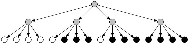
Pretty straightforward, although there’s some not-easy-to-remove repetition. For running on the 4×4 chunk above, it’ll make a tree that looks like this:
Compressing a quadtree
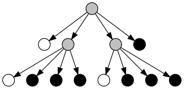
This is where I’m going to depart from the example in the Turing Omnibus. What they do is, when all leaf nodes under a subtree are the same, then that subtree is turned into a leaf node of that color, like so:
What I’m going to do is a little different. I’m going to remove duplicated nodes, so the resulting tree looks like this:
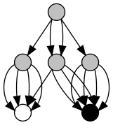
Each node that appears twice (like the two middle children of the root in the original graph) only gets stored once, and we have the root refer to it twice. The way we’ll do this is to work from the bottom up, keeping a list of nodes we’ve seen before (determined with equal). If we don’t find the current node in the list, we add it; then we add its index. What we’re left with is a big list of node definitions, starting with two nodes that just contain “true” and “false”, and ending with a node that represents our whole picture. Here’s the final list for the 4×4 quadrant:
1	false
2	true
3	1	1	1	1
4	1	2	2	2
5	2	2	2	2
6	3	4	4	5
The first column is the index, then there are the four childrens’ indices. You can see how this matches the graph above: the last (root) node contains a node of all white, then two copies of a node with all black except the first one, then a node of all black. Here’s the function to create the compressed tree:
function compress_tree(tree, flyweights)
   flyweights = flyweights or {false, true}

   if type(tree) == 'table' then
      local new_tree = {}
      for k,v in ipairs(tree) do
         new_tree[k] = compress_tree(v, flyweights)
      end
      tree = new_tree
   end

   for index, flyweight in ipairs(flyweights) do
      if equal(tree, flyweight) then
         return index, flyweight
      end
   end

   table.insert(flyweights, tree)
   return #flyweights, flyweights
end
A “flyweight” is any node that appears in multiple places in a tree, reused to save space. We start out by creating a flyweight table containing the two basic nodes, then we look at the current node: if it’s a tree, we recurse on all its children to turn them into node indices. Then, we just need to find where the current node is in the flyweight table, and return that index (and the updated flyweight table). It’s very straightforward, if a little ugly to be passing around and modifying the table.
Some examples
Here’s the function to print out the list of node types:
function print_flyweight_table(flyweights)
   for index, f in ipairs(flyweights) do
      if type(f) == 'table' then
         print(index, f[1], f[2], f[3], f[4])
      else
         print(index, f)
      end
   end
end
Using it, we can easily generate a bunch of tables for different bitmaps. The original upvote arrow becomes:
1	false
2	true
3	1	1	1	1
4	1	2	2	2
5	2	2	2	2
6	3	4	4	5
7	2	1	2	2
8	7	3	5	7
9	1	2	1	2
10	3	9	3	9
11	2	1	2	1
12	11	3	11	3
13	6	8	10	12
Only thirteen nodes, from 64 bits. Since we can pack each node into 16 bits (4 bits per index, 4 indices per node) and only eleven of the nodes need to be packed (the first two aro always the constants), that’s 22 bytes. Which is actually larger than the original bitmap, so that’s not so good. Let’s see if we can do better:
#......#..####..
.#....#..#....#.
..#..#..#......#
...##...#......#
...##...#......#
..#..#..#......#
.#....#..#....#.
#......#..####..
..####..#......#
.#....#..#....#.
#......#..#..#..
#......#...##...
#......#...##...
#......#..#..#..
.#....#..#....#.
..####..#......#

1	false
2	true
3	2	1	1	2
4	1	1	1	1
5	3	4	4	3
6	1	2	2	1
7	4	6	6	4
8	5	7	7	5
9	1	1	1	2
10	2	2	1	1
11	2	1	2	1
12	9	10	11	4
13	1	1	2	1
14	1	2	1	2
15	10	13	4	14
16	1	2	1	1
17	1	1	2	2
18	11	4	16	17
19	2	1	1	1
20	4	14	17	19
21	12	15	18	20
22	8	21	21	8
22 states, meaning 400 bits (at 5 bits per index), or 50 bytes. Since the original image was 256 bits, this is still not great, even though it has a lot of duplication of large structures. So what could be better compressed…
.#.#.#.#
#.#.#.#.
.#.#.#.#
#.#.#.#.
.#.#.#.#
#.#.#.#.
.#.#.#.#
#.#.#.#.

1	false
2	true
3	1	2	2	1
4	3	3	3	3
5	4	4	4	4
This is almost the ideal case. Five states, 36 bits total to encode 64 bits of source. And, if we increased this image to 16×16, we’d only need one more state for it. So little repeating patterns like that work well. Also:
........
........
.....#..
........
........
........
........
........

1	false
2	true
3	1	1	1	1
4	3	3	3	3
5	1	2	1	1
6	3	3	5	3
7	4	6	4	4
This one is exactly as many bits as the uncompressed form, but if we increased it to 16×16 it wouldn’t be. Images with big blocks of whitespace compress very well this way too.
Other tricks
We can easily rotate the image by just re-ordering the children on each node in the list. Much cheaper to rotate it this way than by copying it, and we can even do it in-place. Plus, it becomes very easy to load a single rectangular region of a map: trace down the tree until you get to the chunk you want and then only render that piece. It could be very useful if you’re making a game around very large generated maps.
Anyway, the code is here, play around with it! Even if it’s not so useful as a way to compress things (run-length encoding is more efficient) it’s still a cool way to store things.